Top 35 Machine Learning Engineer Interview Questions and Answers [2026]

TL;DR: Machine learning engineer interviews in 2026 test whether a candidate can find a leak, pick the right metric, and debug a training run, not recite definitions. On the PyTorch side, expect questions on mixed precision, FSDP2 (fully_shard) and torch.compile, plus three version facts: PyTorch 2.14.1 is current, torch.load defaults to weights_only=True, and torch.jit has been deprecated since 2.10.

PyTorch 2.14.0 shipped on September 2, 2026, and changed how autograd assigns gradients at clamp boundaries: clamp_min(x, 0.0) at x = 0 now gives a gradient of 0, not 1.

Small changes like that are why senior ML interviews now ask about training behavior, not only theory. Interviewers also probe leakage, calibration, fine-tuning and experiment design.

The design round has its own ML system design interview guide.

ML Fundamentals

1. Explain the bias-variance trade-off. How do you tell which one you have?

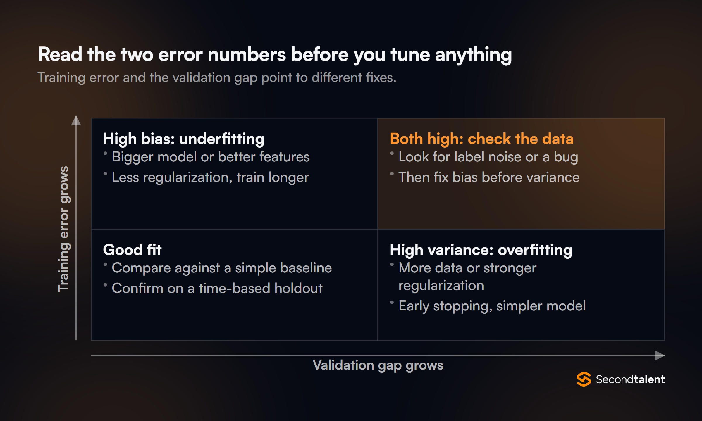
Bias is error from a model too simple to capture the signal; variance is error from a model that fits noise in its training sample. You diagnose it from two numbers: training error, and the gap between training and validation error.

• High training error, small gap: high bias. Add capacity or features, reduce regularization, train longer.
• Low training error, large gap: high variance. Add data, regularize harder, stop earlier or simplify.
• Both high: check the data first. Label noise, a broken join or a preprocessing bug often looks like a modeling problem.

Strong candidates plot learning curves (error against training set size) instead of guessing. If validation error is still falling as data grows, more data will help; if both curves have flattened at a high value, it will not.

2. How do L1 and L2 regularization differ, and is weight decay the same as L2?

L1 adds the sum of absolute weights to the loss and drives some weights to exactly zero, so it also selects features.

L2 adds the sum of squared weights and shrinks all weights smoothly without zeroing them, which handles correlated features better. Elastic net mixes both.

Weight decay equals L2 only for plain SGD. Loshchilov and Hutter showed in Decoupled Weight Decay Regularization that the two are not equivalent for adaptive optimizers such as Adam, because Adam rescales the L2 gradient per parameter.

AdamW applies the decay directly to the weights, outside the adaptive step, which is why it is the default choice for transformers.

3. Which evaluation metric do you choose for an imbalanced classifier?

Start from the cost of each error, then pick the metric. For a fraud model where 0.5% of transactions are positive, accuracy is useless: predicting "not fraud" every time scores 99.5%.

• Precision and recall at a chosen threshold, when the business has a fixed review capacity or a fixed miss tolerance.
• PR AUC (average precision), to compare models across thresholds when positives are rare. Saito and Rehmsmeier showed the precision-recall plot is more informative than ROC on imbalanced data.
• ROC AUC, when you care about ranking quality and classes are not extremely skewed. It can look excellent while precision at the top of the list is poor.
• Log loss or Brier score, when downstream code uses the probability itself, such as expected-value pricing.

The senior follow-up is that the threshold is a business decision, made on a validation set, and reported with the metric.

4. What is data leakage? Give three examples you have seen.

Leakage is any information in training that would not be available at prediction time. The scikit-learn pitfalls guide puts it simply: never call fit on the test data, including inside preprocessing.

• Preprocessing on the full dataset: scaling, imputation or target encoding fitted before the split. Fix it by putting every step in a Pipeline so cross-validation refits it per fold.
• Future information in features: a "days until cancellation" field, or an aggregate computed over a window that ends after the prediction time.
• Duplicates across splits: the same customer, patient or image in train and test, so the model memorizes identities.

The tell is a validation score that is too good. A good candidate looks at the top feature importances first: a single feature carrying most of the signal is usually a leak.

5. How do you handle class imbalance?

Often you do not need to rebalance the data at all. Train on the true distribution with a proper loss, then move the decision threshold. If the minority class is still underfit, use these in order:

1. Class weights (class_weight="balanced" in scikit-learn, pos_weight in BCEWithLogitsLoss). Cheap and keeps all data.
2. Resampling inside each training fold only. Oversampling before the split copies minority rows into the validation set, which is leakage.
3. More minority examples, through labeling or hard-negative mining.

Always evaluate on the untouched, real class ratio. Reweighting and resampling also distort predicted probabilities, so recalibrate afterward if anything downstream reads the score as a probability.

6. What does it mean for a model to be calibrated, and how do you fix one that is not?

A calibrated model's predicted probabilities match observed frequencies: of all cases scored 0.8, about 80% are positive. You check it with a reliability diagram (calibration curve), and measure it with log loss or Brier score.

The scikit-learn calibration guide notes that a lower Brier loss does not by itself mean better calibration, because the score mixes calibration and discrimination.

To fix calibration, fit a calibrator on held-out predictions with CalibratedClassifierCV:

• Sigmoid (Platt): two parameters, safe on small data, assumes a sigmoid-shaped distortion.
• Isotonic: non-parametric and more flexible, but prone to overfitting; the docs say it matches or beats sigmoid with more than about 1,000 samples.
• Temperature: one parameter for all classes, added in scikit-learn 1.8 (question 35).

Calibrating on the training data is the classic mistake: the calibrator learns the model's overconfidence on examples it has already memorized.

7. How do you encode a categorical feature with 50,000 values?

One-hot encoding is out at that cardinality for most models. The common options:

• Target encoding: replace each category with the mean target, smoothed toward the global mean for rare categories. Compute it out-of-fold, or each row's own label leaks into its feature.
• Frequency or count encoding: simple, leak-free, often strong for trees.
• Hashing: fixed memory, tolerates unseen values, accepts collisions.
• Learned embeddings: for neural networks, with an "unknown" bucket for values that appear after training.

Also ask what happens to a category that first appears in production. A candidate who has shipped models will have an answer for unseen values and for categories whose meaning changes over time.

8. Gradient-boosted trees or a deep network for tabular data?

Start with gradient-boosted trees (XGBoost, LightGBM, CatBoost) for typical tabular problems.

In Grinsztajn, Oyallon and Varoquaux's benchmark of 45 datasets, tree-based models remained the best performers on medium-sized data (about 10,000 samples), even before counting their speed advantage.

The authors tie the gap to inductive bias: trees tolerate uninformative features and learn irregular functions easily.

A deep network earns its place when the inputs include text, images or long event sequences, when you need embeddings shared with other models, or when the data is large enough to amortize the tuning.

Many production systems combine the two: neural embeddings as features into a boosted tree.

9. How do you cross-validate when rows are not independent?

Match the split to how production will use the model. Standard k-fold assumes independent, identically distributed rows, which rarely holds in production data.

• Time-ordered data: TimeSeriesSplit trains on earlier folds and tests on the next one. Its gap parameter leaves a buffer so labels that mature late do not leak.
• Grouped data: GroupKFold keeps all rows from one user, patient or device in the same fold, so the score reflects unseen groups.
• Both: split by time first, then make sure no group spans the boundary.

Random k-fold on time series is one of the most common reasons an offline score does not survive launch.

PyTorch Training

10. SGD, Adam or AdamW: which do you use, and with what schedule?

AdamW is the default for transformers and most new deep learning work; SGD with momentum is still competitive for some vision models and often generalizes well once tuned.

Adam keeps two moment estimates per parameter, so it costs 8 extra bytes per parameter in fp32 compared with SGD's 4 for momentum.

The schedule usually matters more than the optimizer. A short linear warmup avoids large, noisy updates while Adam's moment estimates are still poor, then a cosine or linear decay brings the learning rate down.

Strong candidates also exclude biases and normalization weights from weight decay, and know that fused optimizer kernels exist: PyTorch 2.12 added fused=True for Adagrad, joining Adam, AdamW and SGD (2.12 release notes).

11. How does mixed precision training work, and when do you need a GradScaler?

torch.autocast runs selected ops, such as linear layers and convolutions, in a lower-precision type and keeps precision-sensitive ops in float32.

Per the AMP docs, float16 training normally pairs autocast with torch.amp.GradScaler, while bfloat16 uses autocast alone.

Two details separate experienced candidates. Do not call .half() or .bfloat16() on the model when using autocast; the docs say not to. And clip gradients only after scaler.unscale_(optimizer), or the threshold applies to scaled gradients:

scaler = torch.amp.GradScaler("cuda")
for x, y in loader:
    optimizer.zero_grad(set_to_none=True)
    with torch.autocast(device_type="cuda", dtype=torch.float16):
        loss = loss_fn(model(x), y)
    scaler.scale(loss).backward()
    scaler.unscale_(optimizer)                  # gradients back to true scale
    torch.nn.utils.clip_grad_norm_(model.parameters(), max_norm=1.0)
    scaler.step(optimizer)                      # skipped if grads hold inf or NaN
    scaler.update()

12. Your loss turns into NaN after 3,000 steps. How do you debug it?

Find the first step where something becomes non-finite, then work backward. A sequence that finds most causes quickly:

1. Log the gradient norm every step. A norm that climbs for hundreds of steps points to the learning rate or a missing warmup; a single spike points to one bad batch.
2. Check the inputs of the failing batch with torch.isfinite. Corrupt records and division by zero in feature code are common.
3. Check the loss math. log(softmax(x)) written by hand underflows; use log_softmax, CrossEntropyLoss or BCEWithLogitsLoss, which take logits.
4. Check precision. float16 activations overflow above 65,504. Switching to bfloat16 often fixes it outright.
5. Locate the op with torch.autograd.set_detect_anomaly(True) on a small reproduction, or with DebugMode, which PyTorch 2.10 added for tracking dispatched calls and numerical divergence.

Gradient clipping is a mitigation, not a diagnosis. A candidate who only says "add clipping" has not found the bug.

13. How do you implement gradient accumulation correctly?

Divide each micro-batch loss by the number of accumulation steps, call backward() on each, and step the optimizer once per effective batch. Three traps:

• Distributed sync. Skip gradient communication on the non-final micro-steps: no_sync() with DDP, or set_requires_gradient_sync(False) with FSDP2.
• GradScaler. The AMP examples say to keep gradients scaled during accumulation, call unscale_ just before the step, and call update() only once per effective batch.
• Variable-length batches. Averaging a token-level loss per micro-batch and then averaging the micro-batches does not equal the mean over all tokens. Sum the loss and divide by the total token count of the effective batch.

Batch normalization still sees only the micro-batch, so accumulation does not replace a larger batch for models that depend on batch statistics.

14. DDP or FSDP2: how do you decide, and how much memory does each need?

Do the memory math first. Training with Adam in float32 costs about 16 bytes per parameter before activations: 4 for the weight, 4 for the gradient, 8 for the two moment estimates.

A 7B-parameter model needs about 112 GB for that state alone.

DDP keeps a full copy on every GPU, so it only works when that state plus activations fits on one device.

FSDP2 shards parameters, gradients and optimizer state across data-parallel ranks; on 8 GPUs the same 112 GB becomes about 14 GB per GPU, paid for with all-gather and reduce-scatter traffic.

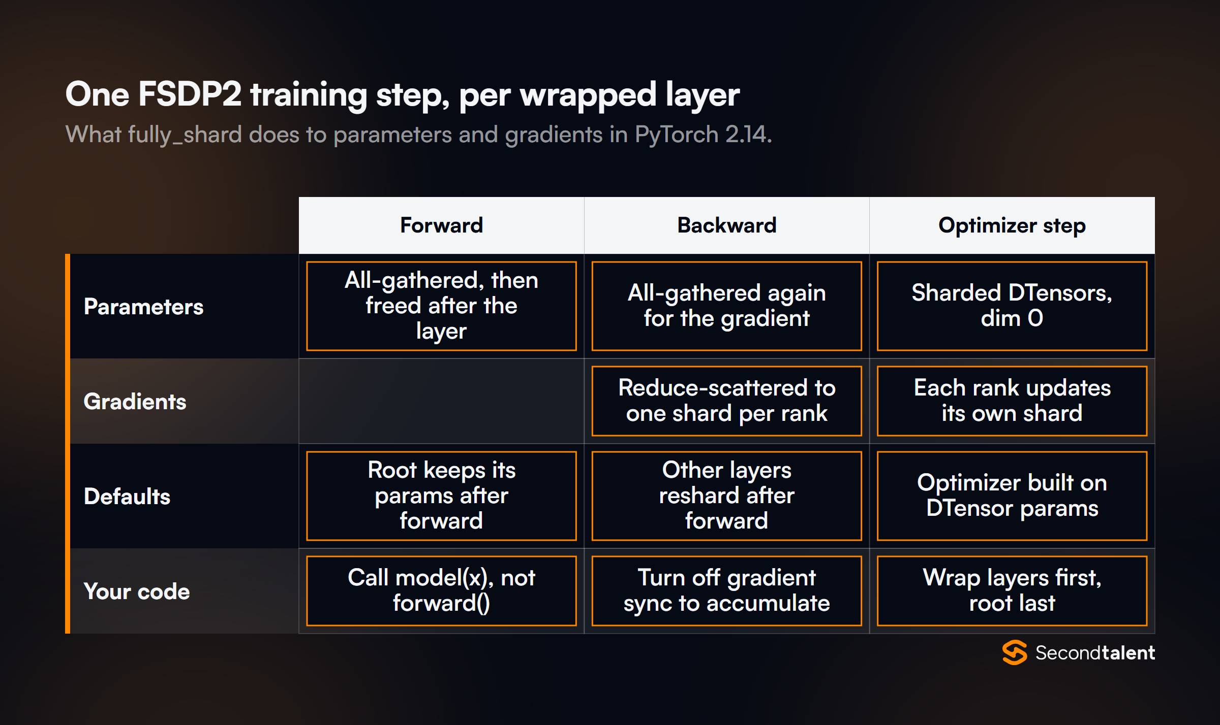
The fully_shard docs give the contract a candidate should know:

• Parameters become DTensors sharded on dim 0, per parameter, unlike FSDP1's flattened groups.
• Apply fully_shard bottom-up: each transformer block first, then the root.
• reshard_after_forward defaults to True for inner modules and False for the root, trading memory for one fewer all-gather.
• Build the optimizer after wrapping, on the DTensor parameters, and call model(x) rather than model.forward(x) so the hooks run.

from torch.distributed.fsdp import fully_shard, MixedPrecisionPolicy

mp = MixedPrecisionPolicy(param_dtype=torch.bfloat16, reduce_dtype=torch.float32)
for block in model.layers:
    fully_shard(block, mp_policy=mp)
fully_shard(model, mp_policy=mp)
optimizer = torch.optim.AdamW(model.parameters(), lr=3e-4)

15. What does torch.compile do, and why would it make training slower?

TorchDynamo captures Python code into graphs and the default Inductor backend generates fused kernels for them. The speedup comes from fewer kernel launches and less memory traffic. It gets slower, or no faster, in three situations:

• Graph breaks. Unsupported Python, data-dependent control flow or .item() calls split the function into pieces with eager code between them. fullgraph=True turns a break into an error so you find it.
• Recompiles. Each guard failure, such as a new input shape, triggers a recompile. Per the torch.compile docs, after recompile_limit (8 by default) the frame falls back to eager. TORCH_LOGS=guards shows why.
• Compile time. Short jobs and evaluation loops may never earn back the compile cost.

Mode matters too: "reduce-overhead" uses CUDA graphs to cut Python overhead for small batches, at the cost of extra memory.

16. What is activation checkpointing, and what does it cost?

It discards intermediate activations during the forward pass and recomputes them during backward, trading compute for memory.

Checkpointing every transformer block reduces activation memory to roughly the block inputs plus one block's internals, and costs about one extra forward pass per step.

Use torch.utils.checkpoint.checkpoint with use_reentrant=False; selective activation checkpointing, which requires that setting, takes a context_fn that decides which op outputs to keep and which to recompute.

A senior candidate reaches for checkpointing after sharding and mixed precision, and measures step time before and after.

17. What changes between model.train() and model.eval()?

The mode switches the behavior of layers such as dropout and batch normalization. In training mode, dropout zeroes activations at random and batch norm normalizes with the current batch's statistics while updating running averages.

In eval mode, dropout is off and batch norm uses the stored running averages.

model.eval() does not turn off gradient tracking; that is torch.no_grad() or torch.inference_mode(), and evaluation code needs both.

Small per-GPU batches make batch statistics noisy, which is one reason transformers use layer normalization, and why multi-GPU convolutional training may need SyncBatchNorm.

Fine-Tuning

18. How does LoRA work, and why does it save memory?

LoRA freezes the pretrained weight matrix W and learns a low-rank update: the layer computes W x + (alpha / r) B A x, where A is r by k and B is d by r, with r much smaller than d. PEFT initializes A with Kaiming-uniform values and B with zeros, so training starts from exactly the base model.

For one 4,096 by 4,096 projection, full fine-tuning trains 16.8 million weights; LoRA with r = 16 trains 131,072, under 1%. Gradients and Adam state exist only for the adapters, which is where the memory goes.

The LoRA paper reports 10,000 times fewer trainable parameters and 3 times less GPU memory than full fine-tuning GPT-3 175B with Adam, with no added inference latency once merged.

19. What does QLoRA add on top of LoRA?

QLoRA stores the frozen base model in 4-bit precision and backpropagates through it into 16-bit LoRA adapters. The QLoRA paper introduced three pieces:

• 4-bit NormalFloat (NF4), a data type designed for normally distributed weights.
• Double quantization, which quantizes the quantization constants too.
• Paged optimizers, which absorb memory spikes.

Together they let the authors fine-tune a 65B model on one 48 GB GPU while matching 16-bit fine-tuning performance on their benchmarks. The trade-off is dequantization work on every forward and backward pass.

Because you trained the adapter against quantized weights, merge it into a 16-bit copy of the base and rerun the evaluation before serving.

20. How do you choose rank, alpha and target modules?

In PEFT's LoraConfig, r and lora_alpha both default to 8, and PEFT scales the update by alpha divided by r. Per the PEFT LoRA guide:

• The default adapters go on the attention query and value layers. target_modules="all-linear" applies LoRA to every linear layer, as QLoRA did, which the guide says can match a fully fine-tuned model.
• use_rslora=True scales by alpha over the square root of r, which keeps higher ranks stable.
• rank_pattern and alpha_pattern set different values per layer.
• merge_and_unload() folds the adapter into the base weights to remove the extra latency at serving time.

A sound process: start with a modest rank on all linear layers, tune the learning rate, and raise rank only if the adapter clearly underfits the task.

21. How do you know a fine-tune actually helped?

Compare it against the cheapest baseline that could have worked, usually the base model with a good prompt or a few examples, on a held-out set built before training. Then check what it broke.

• Task eval: held-out examples from the target distribution, never paraphrases of training rows.
• Regression eval: a fixed set of general tasks the base model handled, to catch catastrophic forgetting.
• Data audit: the QLoRA authors found a small, high-quality dataset beat the previous best results, even with smaller models, so quality beats volume.

Evaluation and monitoring of LLM applications in production belong to the system design round.

Experiments and Drift

22. How do you make a training run reproducible?

Control randomness, force deterministic kernels where you need them, and record everything else.

The PyTorch reproducibility notes are explicit that full reproducibility is not guaranteed across releases, platforms or CPU versus GPU, even with identical seeds.

import random, numpy as np, torch

def seed_everything(seed: int):
    random.seed(seed)
    np.random.seed(seed)
    torch.manual_seed(seed)                     # seeds CPU and all CUDA devices
    torch.backends.cudnn.benchmark = False      # same conv algorithm every run
    torch.use_deterministic_algorithms(True)    # error on nondeterministic ops

def seed_worker(worker_id):
    worker_seed = torch.initial_seed() % 2**32
    np.random.seed(worker_seed)
    random.seed(worker_seed)

g = torch.Generator()
g.manual_seed(0)
loader = torch.utils.data.DataLoader(ds, batch_size=64, num_workers=4,
                                     worker_init_fn=seed_worker, generator=g)

Then pin the environment: library versions, CUDA version, GPU type and count, the data snapshot and the code commit. Deterministic mode is slower, so many teams use it for debugging and regression tests rather than every production run.

23. What do you log for every experiment?

Enough to rebuild the model and to compare it fairly against every other run. In practice that means:

• Hyperparameters and the full config file, not only the values you changed.
• Metrics per step and per epoch, on a versioned evaluation set that stays fixed across runs.
• Code commit, data snapshot or hash, and environment.
• Artifacts: the checkpoint, the preprocessing pipeline and the decision threshold.

Tools such as MLflow, Weights and Biases or a managed equivalent handle this. MLflow 3 made the model itself a first-class record: its release notes introduce a LoggedModel entity that moves tracking beyond the run-centric approach.

MLflow 3.17.1, released October 13, 2026, is current.

24. Two runs with the same seed give different results. Why?

Usually because something other than the seed changed, or a kernel is nondeterministic. Common causes:

• Some GPU operations are nondeterministic; torch.use_deterministic_algorithms(True) makes PyTorch raise an error when one runs.
• cudnn.benchmark=True can pick a different convolution algorithm per run.
• A different GPU count changes reduction order and, often, the effective batch size.
• DataLoader workers without seeded generators shuffle or augment differently.

The deeper point: even a perfectly deterministic pipeline gives one sample from a distribution of outcomes. Before claiming a 0.3-point improvement, a strong candidate runs several seeds of both configurations and compares the spread.

25. The new model wins offline but the A/B test is flat. What happened?

The offline metric did not measure what the online metric rewards, or the test could not see the difference. Work through the causes in order:

1. Metric mismatch: a better AUC on all items does not mean better results in the top 10 slots users actually see.
2. Biased offline data: logs were produced by the old model, so they contain few examples of what the new model would show.
3. Leakage or a stale split made the offline gain partly fake (question 4).
4. Latency: a slower model can lose online what it gains in quality.
5. Power: the test was too small to detect an effect of the size offline predicted.

The fix is to build an offline metric that tracks past online results, then trust it more each time it predicts correctly.

26. How do you size and run an A/B test for a model change?

Fix the primary metric, guardrail metrics and minimum detectable effect before launch, then compute the sample size.

For 80% power at a two-sided 5% significance level, a standard approximation is n per arm = 16 times the variance divided by the squared effect size.

For a 5% conversion rate and a 0.25-point absolute lift (5% relative), the variance is 0.05 times 0.95, so n = 16 x 0.0475 / 0.0025², about 121,600 users per arm. That number decides how long the test runs. Then:

• Randomize on the unit that matters (user, not request) so one user sees one model.
• Do not stop early on a significant result unless you use a sequential testing method; repeated peeking inflates false positives.
• Run full weekly cycles, and watch for novelty effects that fade.
• Check the traffic split. A 50/50 test that lands at 52/48 signals a bug in assignment or logging.

27. How do you decide when to retrain a model?

Measure how fast the model decays, then set the cadence from that, not from habit. Backtest: train on data up to several past dates and score each model on the weeks that followed.

The curve of metric against model age tells you whether weekly, monthly or quarterly retraining pays for itself.

• Scheduled retraining suits steady decay.
• Triggered retraining suits sudden shifts, such as a pricing change or a new market, once labeled data from the new regime exists.
• Warm start versus from scratch: fine-tuning the last model is cheaper but can carry old bias forward; retrain from scratch periodically to compare.

Every retrained candidate should beat the current model on a fixed holdout and on the most recent window before it ships. The system design guide linked above covers drift detection and rollout mechanics.

Coding Round

28. Implement ROC AUC without a library.

Use the rank formulation: AUC is the probability that a random positive scores higher than a random negative, with ties counting half. Sorting makes it O(n log n) instead of comparing every pair.

def roc_auc(y_true, scores):
    pairs = sorted(zip(scores, y_true))
    n = len(pairs)
    ranks = [0.0] * n
    i = 0
    while i < n:                      # average ranks across tied scores
        j = i
        while j + 1 < n and pairs[j + 1][0] == pairs[i][0]:
            j += 1
        for k in range(i, j + 1):
            ranks[k] = (i + j) / 2 + 1
        i = j + 1
    n_pos = sum(y for _, y in pairs)
    n_neg = n - n_pos
    if n_pos == 0 or n_neg == 0:
        raise ValueError("AUC needs both classes")
    pos_rank_sum = sum(r for r, (_, y) in zip(ranks, pairs) if y == 1)
    return (pos_rank_sum - n_pos * (n_pos + 1) / 2) / (n_pos * n_neg)

print(roc_auc([0, 0, 1, 1], [0.1, 0.4, 0.35, 0.8]))   # 0.75
print(roc_auc([0, 1, 0, 1], [0.5, 0.5, 0.2, 0.9]))    # 0.875, the tie counts half

Interviewers look for tie handling, the single-class edge case, and an explanation of why AUC ignores calibration: any monotonic transform of the scores gives the same answer.

29. Write a numerically stable softmax cross-entropy.

Subtract the maximum logit before exponentiating (the log-sum-exp trick). The result is mathematically identical and never overflows.

import math

def cross_entropy(logits, target):
    m = max(logits)
    log_sum_exp = m + math.log(sum(math.exp(z - m) for z in logits))
    return log_sum_exp - logits[target]

print(cross_entropy([2.0, 1.0, 0.1], 0))   # 0.417
print(cross_entropy([1000.0, 0.0], 1))     # 1000.0; the naive version raises OverflowError

The follow-up: this is why PyTorch's CrossEntropyLoss takes raw logits. Applying softmax in the model and then passing probabilities to it applies softmax twice, a silent bug that raises no error.

30. Find the bugs in this training loop.

This is a common live exercise. The loop runs without errors, which is what makes it a good test.

model.train()
for epoch in range(epochs):
    total = 0
    for x, y in loader:
        loss = loss_fn(model(x), y)
        loss.backward()
        optimizer.step()
        total += loss
    acc = evaluate(model, val_loader)

def evaluate(model, loader):
    model.eval()
    correct = 0
    for x, y in loader:
        correct += (model(x).argmax(-1) == y).sum()
    return correct / len(loader)

• No optimizer.zero_grad(): gradients accumulate across every step.
• total += loss keeps each step's autograd graph alive, so memory grows all epoch. Use loss.item().
• model.train() sits outside the loop: after the first evaluate call, every later epoch trains in eval mode with dropout off and frozen batch norm statistics.
• No torch.no_grad() in evaluation, so it builds graphs it never uses.
• len(loader) counts batches, not examples. Divide by len(loader.dataset).

Strong candidates also ask whether loss_fn expects logits and whether the last batch is smaller than the rest. We ran the plain Python snippets in this section as written; the PyTorch loop is illustrative.

What Changed Recently

31. Old checkpoints fail to load after a PyTorch upgrade. Why?

Since PyTorch 2.6, torch.load defaults to weights_only=True.

Per the 2.6 release notes, it now uses a restricted unpickler that only loads state dictionaries and basic types, so a checkpoint that pickled a whole model object or a custom config class raises an error.

The right fixes, per the serialization notes: save state_dict() rather than the module, or allowlist specific classes with torch.serialization.add_safe_globals.

Passing weights_only=False is acceptable only for files you fully trust, because unpickling can run arbitrary code. For checkpoints from outside your organization, the release notes point to safetensors.

32. What replaces TorchScript?

torch.compile for speeding up Python training and inference, and torch.export for capturing a graph to run elsewhere.

The 2.10 release notes added deprecation warnings to the user-facing torch.jit API, state that it is not guaranteed to work on Python 3.14, and name those two as replacements.

ONNX export moved the same way: 2.11 removed the fallback option that silently retried with the TorchScript-based exporter when the dynamo exporter failed.

A candidate maintaining torch.jit.script models should have a migration plan, not just a pinned version.

33. What did PyTorch 2.13 change for large-model training?

Two changes matter in interviews. Per the 2.13 release notes, released July 8, 2026:

• FSDP2 communication overlap: FSDPModule.set_separate_reduce_scatter_group gives reduce-scatter its own NCCL communicator, so it can overlap with all-gather. It is opt-in.
• nn.LinearCrossEntropyLoss fuses the final projection with the loss, cutting peak GPU memory by up to 4 times for large-vocabulary language model training, because the full logits tensor is never stored at once.

2.13 also gave FlexAttention a deterministic backward path on CUDA, which helps the reproducibility work in question 22. In 2.14, LinearCrossEntropyOptions dropped acc_policy="balanced"; code that set it must switch to "compact".

34. A model retrained on PyTorch 2.14 behaves slightly differently. What could it be?

One candidate is the autograd change in the 2.14 release notes: clamp and min/max subgradients at exact boundaries changed. With a scalar bound, the gradient at equality is now 0 instead of 1.

With a tensor bound, clamp, clamp_min and clamp_max split the gradient evenly between input and bound at a tie, where 2.13 gave it all to the input.

x = torch.tensor(0.0, requires_grad=True)
torch.clamp_min(x, 0.0).backward()
print(x.grad)   # 2.13: tensor(1.)   2.14: tensor(0.)

Values that sit exactly on a bound are common with ReLU-like clamps, quantized inputs and clipped features, so the change can move results. Code that needs the old behavior can write it explicitly with torch.where.

The same release also deprecates the default for selective activation checkpointing with saved-tensor hooks, so watch for a new FutureWarning.

35. What is temperature scaling, and when do you use it over isotonic calibration?

Temperature scaling divides the logits by a single learned value T before the softmax.

It changes confidence without changing the predicted class. scikit-learn 1.8, released December 10, 2025, added it as CalibratedClassifierCV(method="temperature").

The 1.8 release highlights explain the advantage for multiclass problems: one parameter in total, where sigmoid and isotonic calibration fit one-vs-rest calibrators that add parameters per class.

Use temperature for multiclass models and small calibration sets; use isotonic when you have plenty of data and the distortion is not monotonic in a simple way. scikit-learn 1.9.1 is current.

Signs of a Strong Answer

• They ask how the model's output will be used before naming a metric, and they set the threshold on validation data.
• They look for leakage first when a score looks too good, starting from the top feature importances.
• They do memory math (bytes per parameter times parameter count) before choosing DDP, FSDP2 or LoRA.
• They know where unscale_, zero_grad and model.train() go without looking it up.
• They report results across several seeds and compute A/B test sample sizes before launch.
• They can name what changed in the PyTorch version they use, such as the weights_only default or the torch.jit deprecation.

Hiring ML Engineers

Engineers who can both debug a distributed training run and design a sound experiment are hard to screen through resumes alone.

Second Talent helps US startups hire vetted AI-Native Engineers from Asia, including machine learning engineers, at $29 to $39 USD an hour billed monthly, with a 90-day one-time replacement guarantee.

See what an ML engineer costs or read the machine learning engineer role guide.

Tell us the stack and we match you with candidates in 24 hours. Start hiring.